Building an xG model with machine learning

When it comes to analysis in football (soccer), the statistic that has become very popular is expected goals (xG). These models have become used in almost every analysis you see from public to club level.

For most people, it is just a black box of what goes into the models. I assume most people understand that location is an important factor but that’s probably about it.

When watching matches it’s funny to hear announcers say “Why is that a .05 xG shot? That should be .5 xG!”.

The models can be trained with a lot of different “features” also known as “input variables”. In the shot above the shot had a 9.2% goal probability (so about a .092 xG). This could be taking into account:

• position

• defenders positioning

• type of play

• foot/body part used

• goal position

• angle

• distance

• etc.

There are a ton of variables that can go into the model.

The hard part about these models is that the best ones need a lot of data and a lot of input variables to get the best results.

Since most likely you are like me and don’t work at one of the big data companies or work at a club, we have to work with scraped data that we’ve gathered, which I used the method & code from my Sports Data Webscraping Workshop to gather the data.

In this article, let’s dive through the actual coding of an xG model by using machine learning.

1. Data Exploration and Cleansing

The first part of building and training any machine learning model is to understand the data that is going into it.

I’m going to load my data and take a look at the first couple of rows:

You can see we have a lot of data points here, we have x and y coordinates, and we have what is going to be our target variable: is_goal, or in other words this is the variable we are trying to predict.

An xG model is slightly different as to get the xG values, we look at the probability of our prediction of is_goal being correct.

Right now we have 8118 rows and 25 columns of data. I’d like to reiterate that this is barely enough to train an xG model. Ideally, we’d have millions of rows and hundreds of columns to work with. But since this is for demonstration this is what we’ve got haha.

Here are all of our columns:

We have some pretty go inputs though such as a lot of styles of plays, if it’s a penalty, big chance, which foot, maybe it’s a header.

I’m going to drop a couple of them just because I don’t think they will provide a lot of value:

1. DirectFreeKick

2. DirectCorner

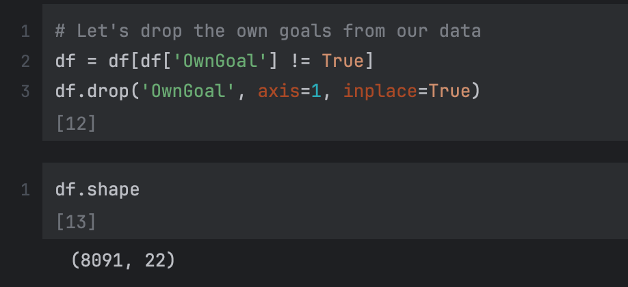
3. OwnGoal

We have to drop all rows that are an OwnGoal because technically those don’t have xG values.

So after dropping some columns and rows, we are down to 8091 rows and 22 columns.

There are a lot of things we can do in data exploration and cleansing. A couple of really important ones are:

• Handling null or missing values

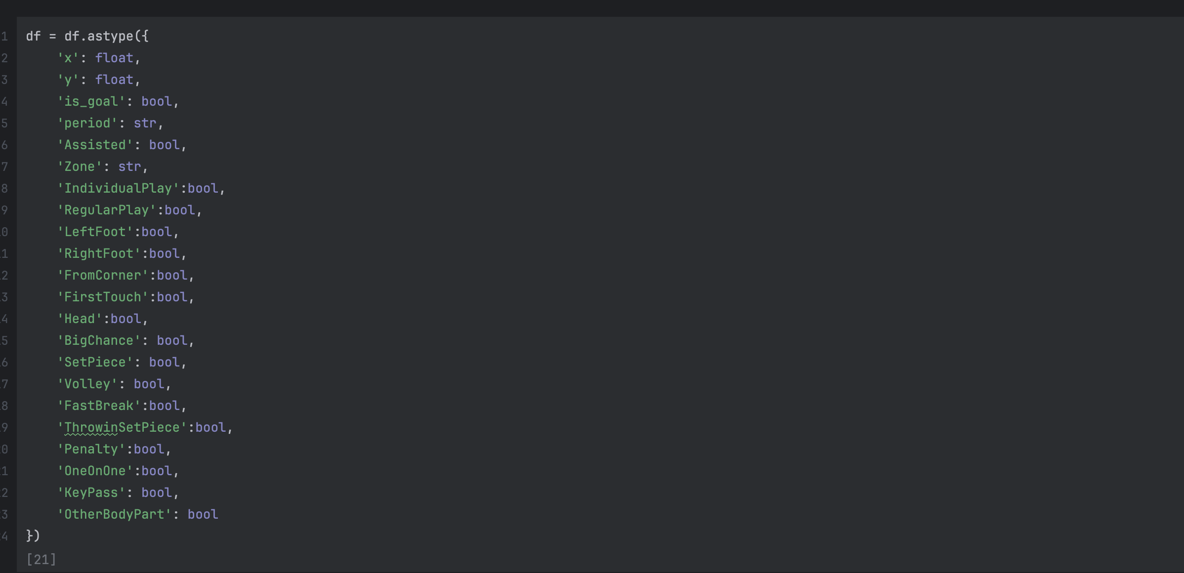
• setting our inputs to the correct data types

So we’ll want to update our null values to be False, we do this because the values only have True or null, so we will fill the nulls with False, and then as well cast our columns to the correct data types.

2. Feature engineering

A common piece of a machine learning workflow is to do something called "feature engineering” where we can update any of our string variables as well as we can come up with new ways to create new variables.

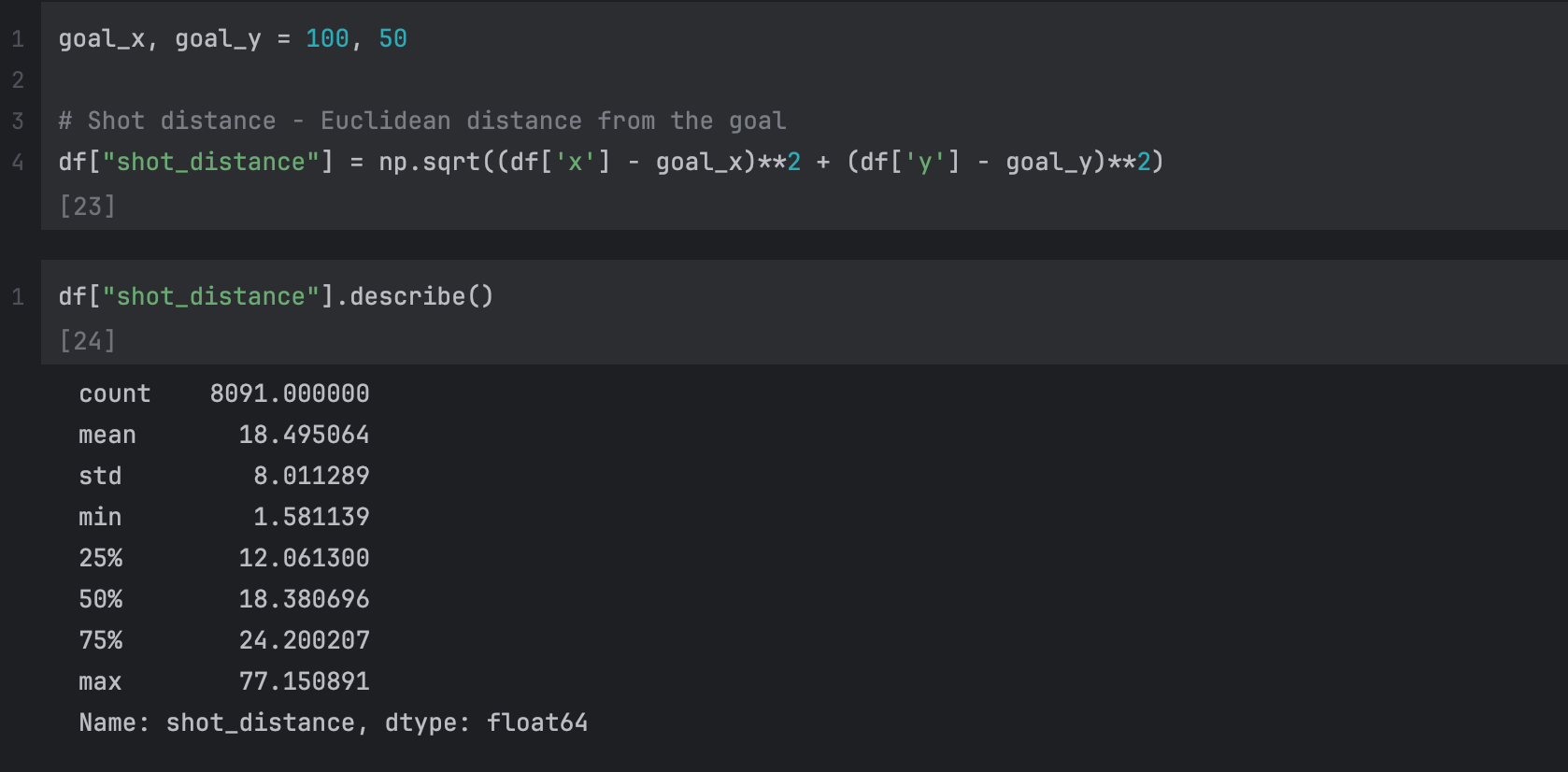
For example, we can create a shot_distance column which allows the model to understand how far away a shot is.

We also can do something called categorical encoding which is the process of updating our string columns like Zone and period, and turning those into separate columns that the model can understand. Most models can’t understand string variable types so with categorical encoding we take all of the different types and create boolean columns for each value in a string column.

Here is the code for calculating the Euclidean distance from the goal:

And here is how we would encode the categorical values:

Notice how we no longer have a “Zone” or a “period” column. Those have been converted into different columns like period_FirstHalf which represent a boolean of if it was True or False for the original period column.

3. Training and testing

We’ll use a Logistic Regression model, which I outline in this other article. The code is straightforward for the first iteration:

Our features/input variables are defined by X while our target variable is y.

We then split the data into training and testing data and then we can train the model by saying model.fit() and then passing in our training data.

Now that we have trained a model, we can make predictions with our test data

We have now successfully trained the model!

These y_pred_proba values are the xG values for the shot in our test data.

We can get some scores about our model which say it is a decent model (there’s room for improvement) but overall it looks like a good starting spot.

And this is what it looks like plotted out

As you can see, we have a good starting spot for training a model. Like I mentioned at the beginning, this model is mainly trained for demonstration purposes as to get a really good model, we’d need more data and could spend a lot more time on the feature engineering and fine-tuning the model.