The Math Behind Expected Goals

Expected goals have changed the way we analyze football, and it has become the metric that has pioneered advanced stats into the public realm.

Expected Goals (xG) quantifies scoring opportunities' quality and provides deeper insights into team and player performances.

Although this metric is widely used, it is less often understood how it actually works behind the hood and its mathematics.

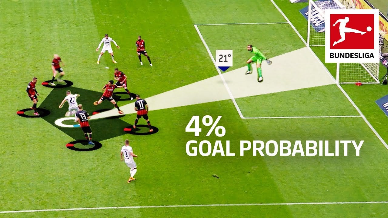
For example in this image, most people watching this match would have no idea how they came up with a 4% goal probability. Even the match commentators don’t really understand it and often question the number they see on screen.

In this newsletter, we'll explore

• the mathematics behind xG

• how it's calculated

• understand why it's become an essential tool in modern soccer analytics

---

What Are Expected Goals (xG)?

Expected Goals is a metric that assigns a probability value to every shot, indicating the likelihood of it resulting in a goal. This value ranges from 0 to 1:

• 0: No chance of scoring.

• 1: Certain goal.

For example, a penalty kick has an xG value around 0.76, meaning there's a 76% chance the penalty will be scored based on historical data.

In reality, you probably won’t see a shot be a flat 0 or 1.

---

The Mathematical Foundation of xG

To understand how xG is calculated there’s a couple of things that you need to understand about creating mathematical and machine learning models.

Every model has training data which is used to learn from historical data and train the model. Each variable of the training data helps the model understand situations to make outputs and predictions.

1. Data Collection

To calculate xG, vast amounts of data are collected for each shot, including:

• Location: Distance and angle relative to the goal.

• Type of Play: Open play, set-piece, counter-attack, etc.

• Body Part Used: Foot, head, other.

• Assist Details: Type of pass leading to the shot.

• Defensive Pressure: Number of defenders nearby.

2. Statistical Modeling

Logistic Regression is commonly used to model xG because the outcome (goal or no goal) is binary, meaning the output is 0 (no goal) or 1 (goal).

The logistic regression equation:

\(P(\text{Goal}) = \frac{1}{1 + e^{-(\beta_0 + \beta_1 x_1 + \beta_2 x_2 + \dots + \beta_n x_n)}} \)

• P(Goal): Probability of the shot resulting in a goal.

• e: Euler's number, base of the natural logarithm, is ~ equal to 2.71828.

• β0​: Intercept term.

• βi: Coefficients for each variable.

• xi​: Variables influencing shot success.

3. Common Key Variables Influencing xG

• Shot Distance: Closer shots have higher xG.

• Angle to Goal: Central angles increase scoring probability.

• Type of Shot: Headers generally have lower xG than shots with the foot.

• Defensive Pressure: More defenders decrease xG.

• Assist Type: Through balls and crosses can increase xG.

Each data provider will train their models with different metrics and variables, and if you train your own you can work with different inputs to see what gives you the most accurate representation.

---

Calculating xG: An Example

Scenario: A player takes a shot from 12 meters out, at a 30-degree angle, with their foot, following a through ball, with one defender nearby.

Step 1: Assign Variable Values

• Shot Distance (x1​) = 12 meters

• Angle to Goal (x2​) = 30 degrees

• Shot Type (x3​) = Foot (1 if foot, 0 otherwise)

• Defensive Pressure (x4​) = 1 defender

• Assist Type (x5​) = Through ball (1 if yes, 0 otherwise)

Step 2: Use Hypothetical Coefficients

Let's assume the following coefficients based on historical data:

• β0​ (Intercept) = -1.2

• β1​ (Distance) = -0.1

• β2​ (Angle) = -0.05

• β3​ (Shot Type) = 0.4

• β4​ (Defensive Pressure) = -0.3

• β5​ (Assist Type) = 0.5

Step 3: Plug Values into the Equation

Calculate the log-odds (logit):

This is a linear combination of the input variables and their coefficients.

\(\text{Logit}(P) = -1.2 + (-0.1 \times 12) + (-0.05 \times 30) + (0.4 \times 1) + (-0.3 \times 1) + (0.5 \times 1) \)

Simplify:

\(\text{Logit}(P) = -1.2 - 1.2 - 1.5 + 0.4 - 0.3 + 0.5 = -3.3 \)

The log-odds transform the probability (which ranges between 0 and 1) to a continuous scale from −∞ to +∞.

Step 4: Convert Logit to Probability

After calculating the log-odds, we convert it back to a probability using the logistic function:

\(P = \frac{1}{1 + e^{-\text{Logit}(P)}} \)

With our values:

\(P(\text{Goal}) = \frac{1}{1 + e^{-(-3.3)}} = \frac{1}{1 + e^{3.3}} \approx \frac{1}{1 + 27.11} \approx 0.035 \)

Result: The shot has an xG value of 0.035, or a 3.5% chance of resulting in a goal.

---

Interpreting xG Values

• Underperformance: Scoring fewer goals than xG suggests may indicate poor finishing or bad luck.

• Overperformance: Scoring more goals than xG predicts could point to exceptional finishing or good fortune.

Example:

• Team A's xG: 2.5

• Actual Goals: 1

Interpretation: Team A underperformed; they created chances but didn't convert.

---

Why Is xG Important?

• Performance Analysis: xG helps evaluate whether a team's performance is sustainable or if they've been lucky/unlucky.

• Player Evaluation: Assesses a player's finishing ability relative to the quality of chances they receive. A typical visualization is to use a shotmap like this one from understat where shots are scaled to their xG value.

  

• Tactical Insights: Informs coaching decisions by highlighting how often a team creates high-quality chances.

---

Limitations of xG

• Data Quality: xG accuracy depends on the detail and reliability of collected data.

• Model Variations: Different providers use different models; xG values can vary. That is why you might see Sofascore have a shot at .32 xG while on Sky Sports they said it was .25.

• Contextual Factors: It usually doesn't fully account for player skill, weather conditions, or specific in-game situations.

---

Expected Goals is a powerful metric and one that can help us understand a lot more about the game.

If you can understand the math behind it, then it can help take your analysis even further.